使用 ggplot2 进行数据可视化
1
2
| # 准备需要用到的包
library(ggplot2)
|
facet_wrap(~ class) 按 class 单个变量分面;facet_grid(drv ~ cyl) 按 drv 和 cyl 两个变量分面
几何对象是图中用来表示数据的几何图形对象。我们经常根据图中使用的几何对象类型来描述相应的图。例如,条形图使用了条形几何对象,折线图使用了直线几何对象,箱线图
使用了矩形和直线几何对象。散点图打破了这种趋势,它们使用点几何对象。
要想改变图中的几何对象,需要修改添加在 ggplot() 函数中的几何对象函数,如 geom_point()、geom_smooth()。ggplot2 中的每个几何对象函数都有一个 mapping 参数,通过 aes() 函数生成参数,如 mapping = aes(x = displ, y = hwy)。
通过分配分类变量(如下面的 linetype = drv),可以对一个几何对象进行分组:
1
2
| ggplot(data = mpg) +
geom_smooth(mapping = aes(x = displ, y = hwy, linetype = drv))
|
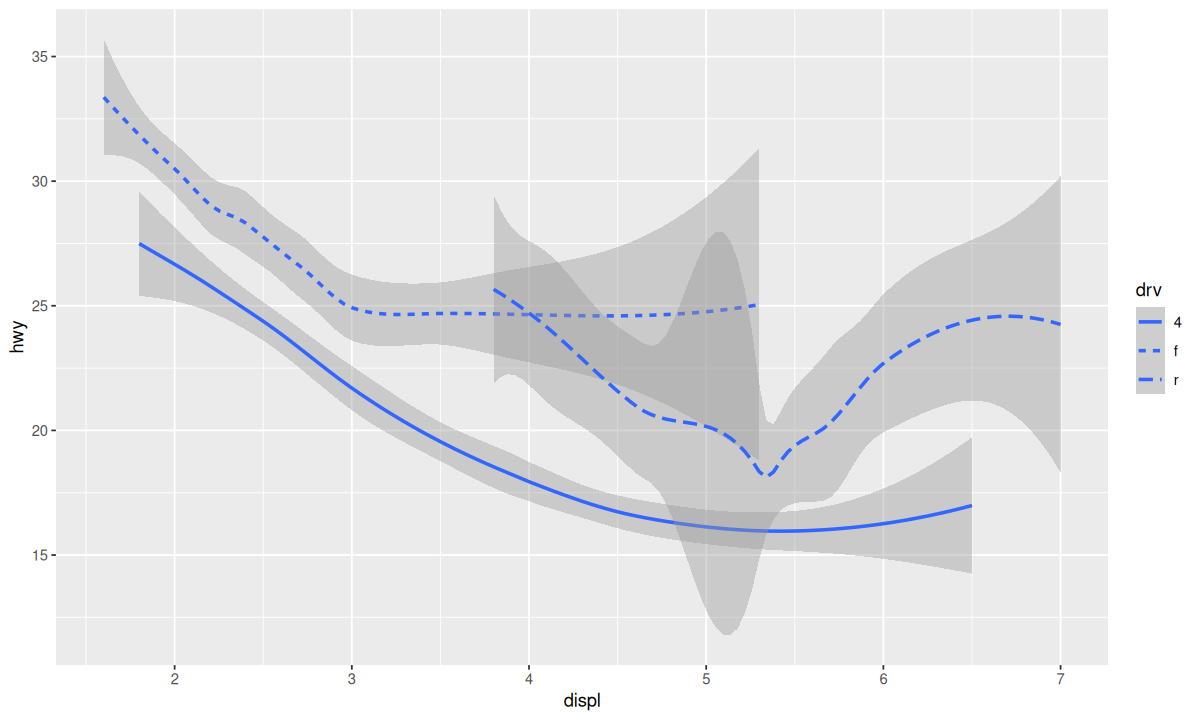
常用的分类变量包括 linetype、color、shape、group 等。
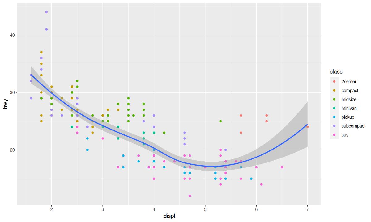
使用全局映射可以方便修改映射,避免遗漏;使用局部映射则可对单个几何对象函数进行修改,实现更细致的操作。
1
2
3
| ggplot(data = mpg, mapping = aes(x = displ, y = hwy)) +
geom_point(mapping = aes(color = class)) +
geom_smooth()
|
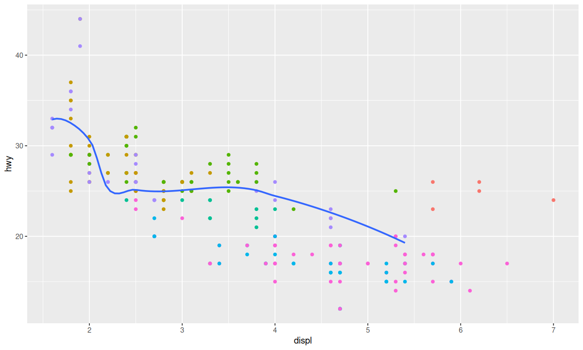
甚至可以为不同的几何对象函数指定不同的数据:
1
2
3
4
5
6
| ggplot(data = mpg, mapping = aes(x = displ, y = hwy)) +
geom_point(mapping = aes(color = class), show.legend = FALSE) +
geom_smooth(
data = dplyr::filter(mpg, class == "subcompact"),
se = FALSE
)
|
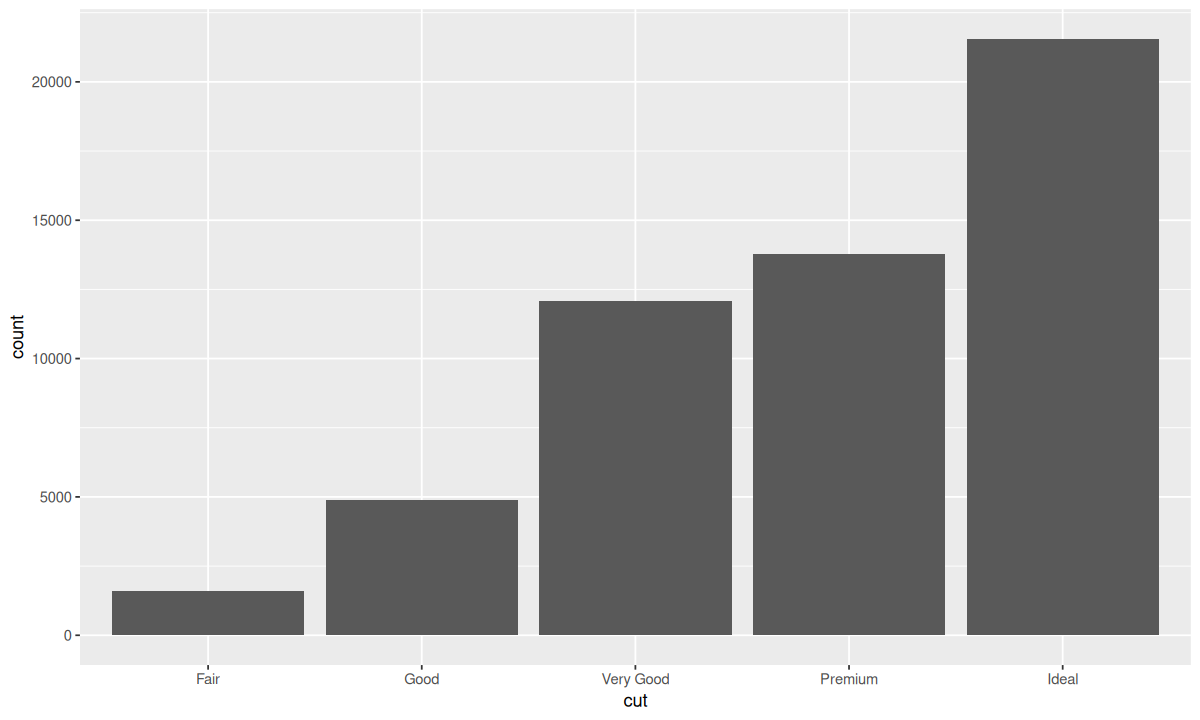
统计变换statstatistical transformation
有些几何对象函数可以计算并绘制出新数据,比如 geom_bar()。
1
2
| ggplot(data = diamonds) +
geom_bar(mapping = aes(x = cut))
|

Y 轴的 count 即为计算出的新变量,而这里使用的统计变换仅是简单的计算数量。查看 ?geom_bar,可以看到 stat 参数的默认值为 "count";而查看 ?stat_count 会发现,显示的页面即为 ?geom_bar 的页面,且 stat_count() 的 geom 默认参数为 bar,其实两者是等价的,所以你还可以这样写:
1
2
| ggplot(data = diamonds) +
stat_count(mapping = aes(x = cut))
|
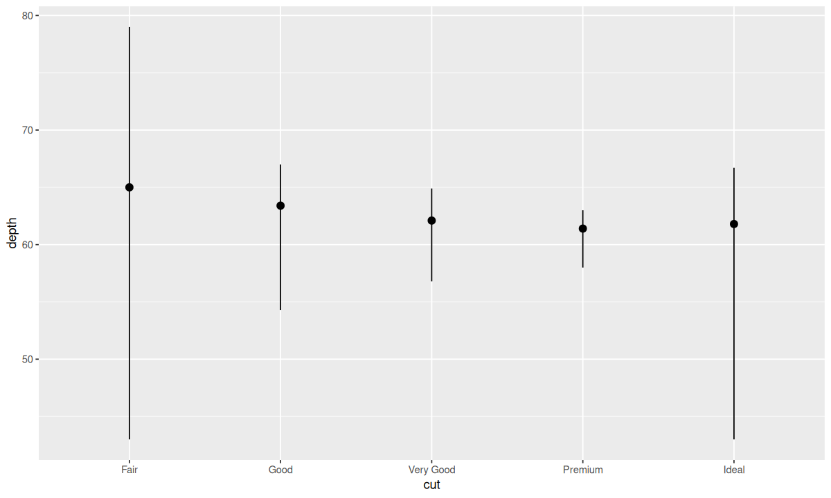
有些 stat 函数没有对应的几何对象函数,如 stat_summary():
1
2
3
4
5
6
7
| ggplot(data = diamonds) +
stat_summary(
mapping = aes(x = cut, y = depth),
fun.min = min,
fun.max = max,
fun = median
)
|
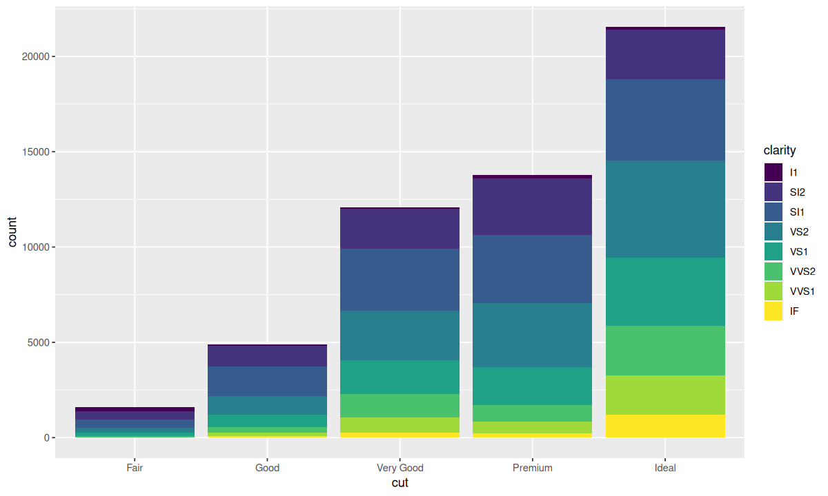
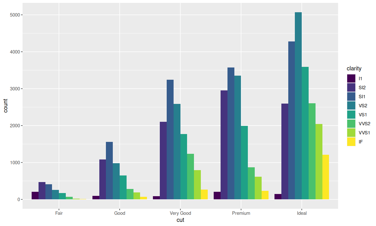
为 geom_bar() 的 fill 参数指定不同的变量可以让条形会自动分块堆叠起来:
1
2
| ggplot(data = diamonds) +
geom_bar(mapping = aes(x = cut, fill = clarity))
|
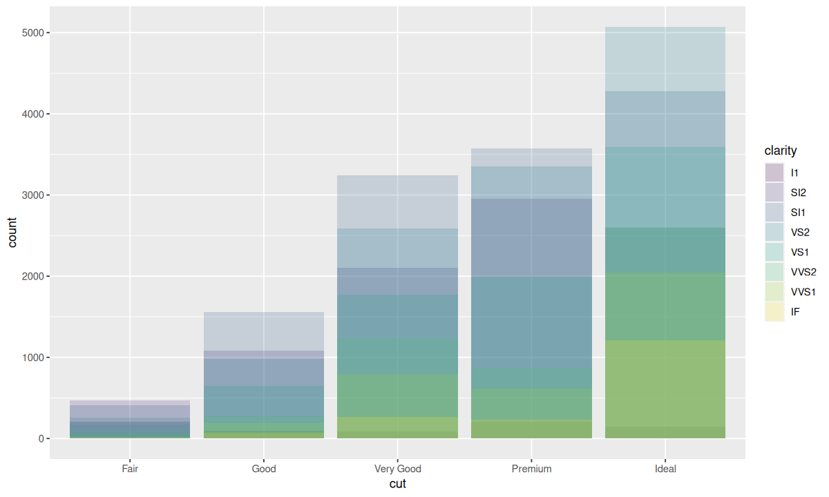
这种堆叠是由 position 参数设定的位置调整功能自动完成的,即 position 的默认值 "stack"。此外,还可以为 position 指定其他值,包括 "identity"、"fill"、"dodge"。
 1
 2
 3
 4
 5
 6
 7
 8
 9
10
11
12
13
14
15
16
17
| ggplot(
data = diamonds,
mapping = aes(x = cut, fill = clarity)
) +
geom_bar(alpha = 1 / 5, position = "identity")
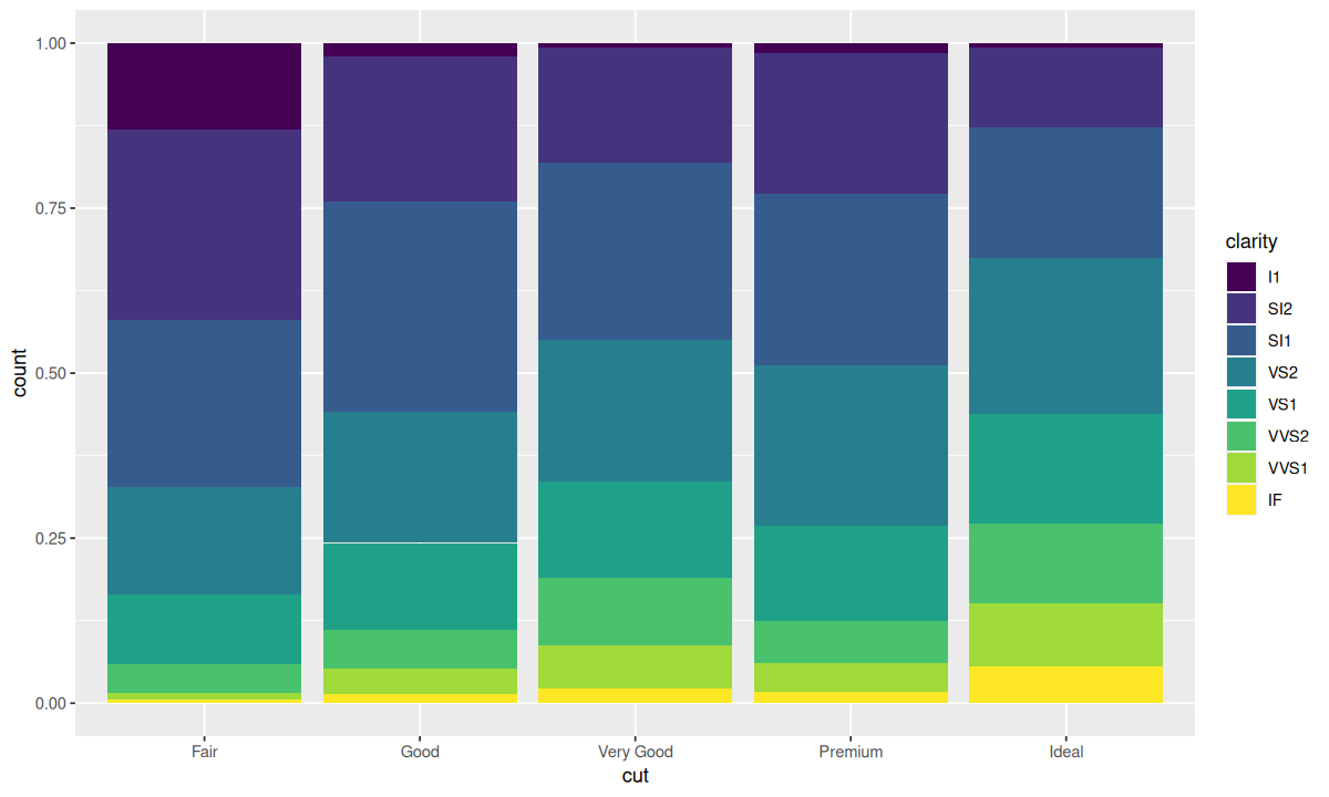
ggplot(data = diamonds) +
geom_bar(
mapping = aes(x = cut, fill = clarity),
position = "fill"
)
ggplot(data = diamonds) +
geom_bar(
mapping = aes(x = cut, fill = clarity),
position = "dodge"
)
|
还有一种位置调整方式——"jitter"(抖动):
1
2
3
4
5
| ggplot(data = diamonds) +
geom_bar(
mapping = aes(x = cut, fill = clarity),
position = "jitter"
)
|
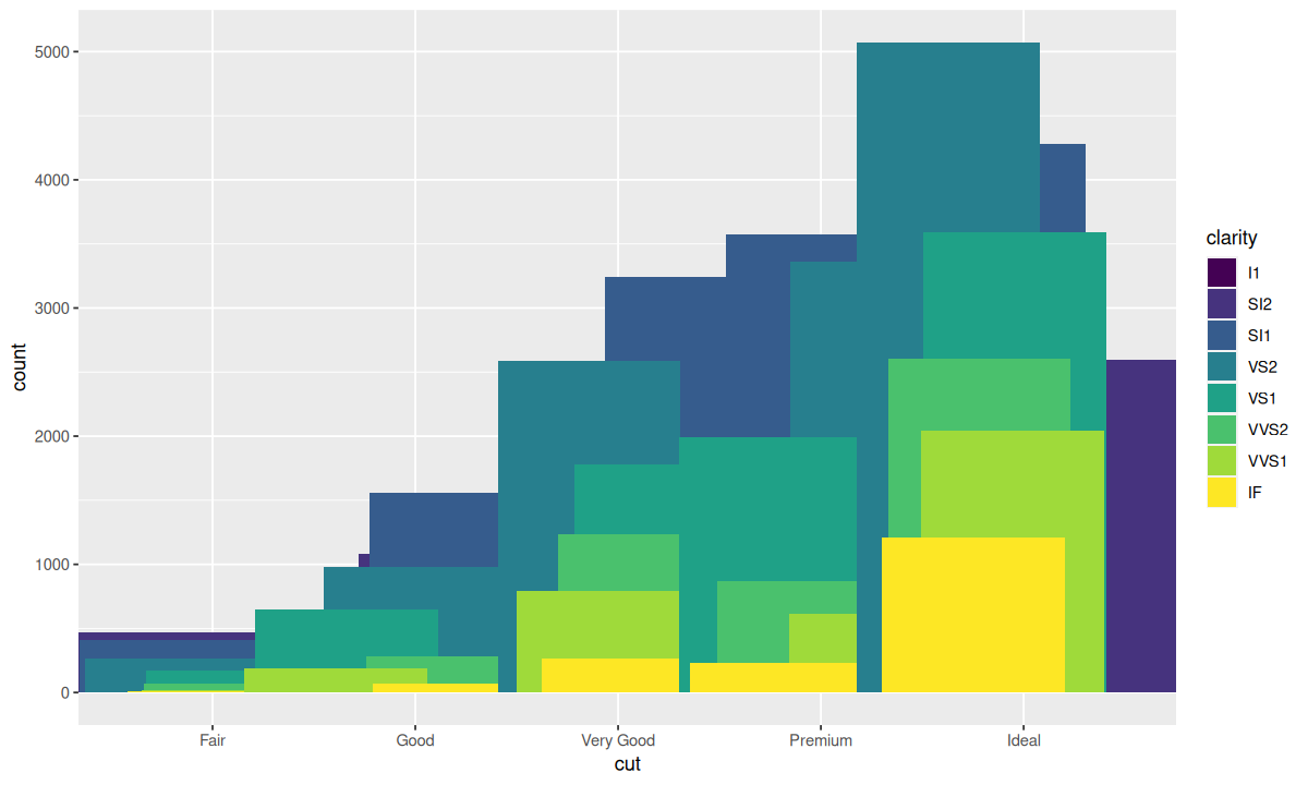
这种位置调整方式更适用于散点图,可以为每一个点添加一个随机的“抖动”避免存在过多点时,点彼此重叠,影响对分布密度的直观判断。
1
2
3
4
5
| ggplot(data = mpg) +
geom_point(
mapping = aes(x = displ, y = hwy),
position = "jitter"
)
|
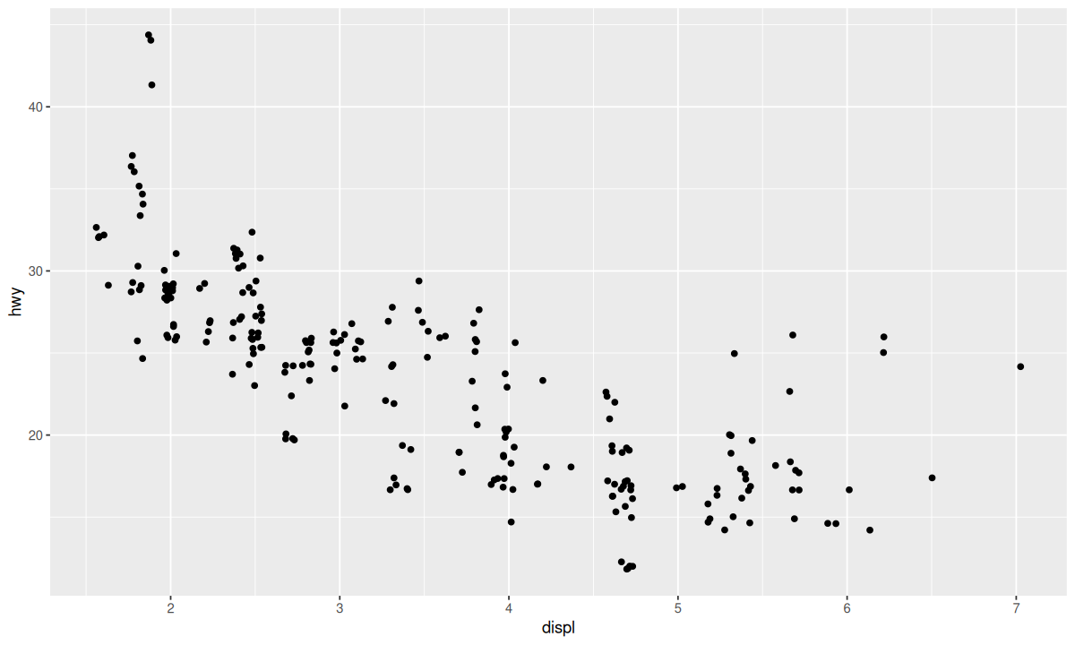
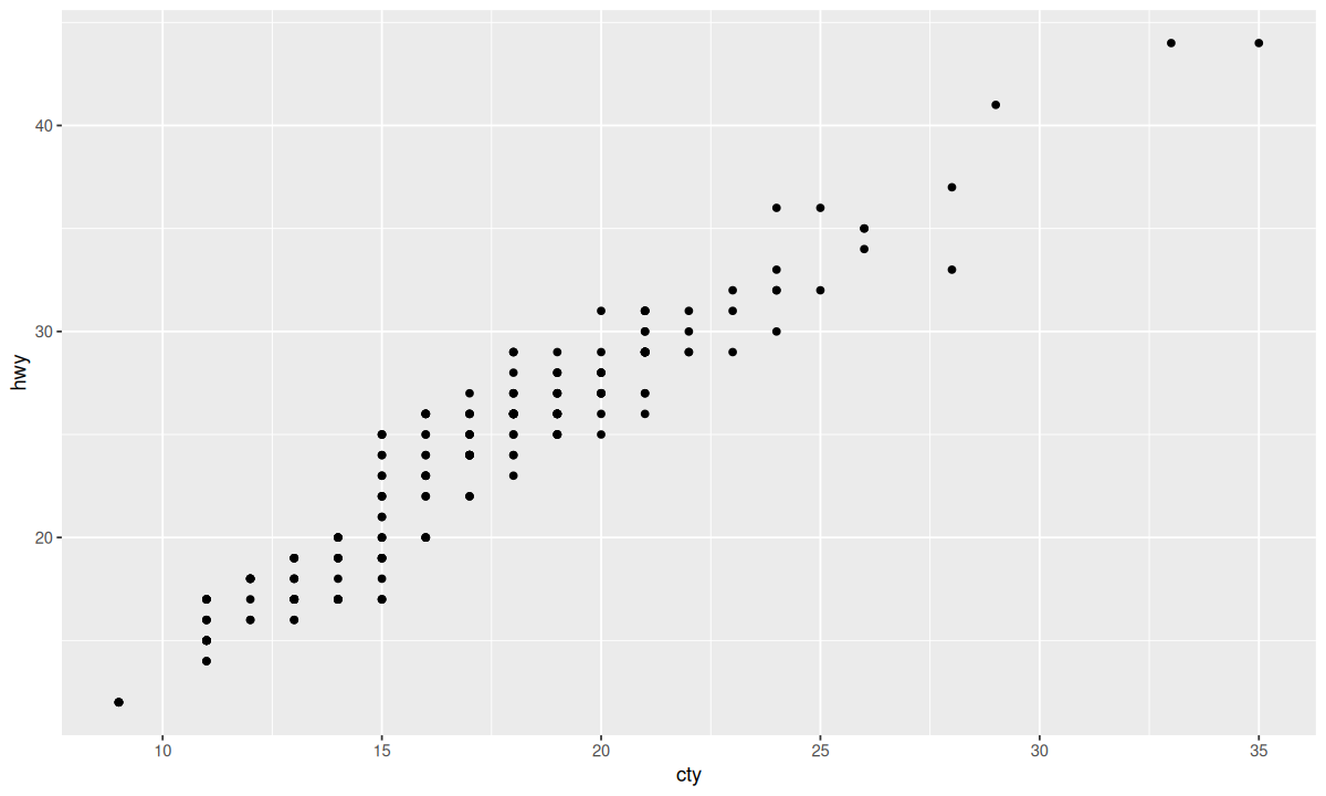
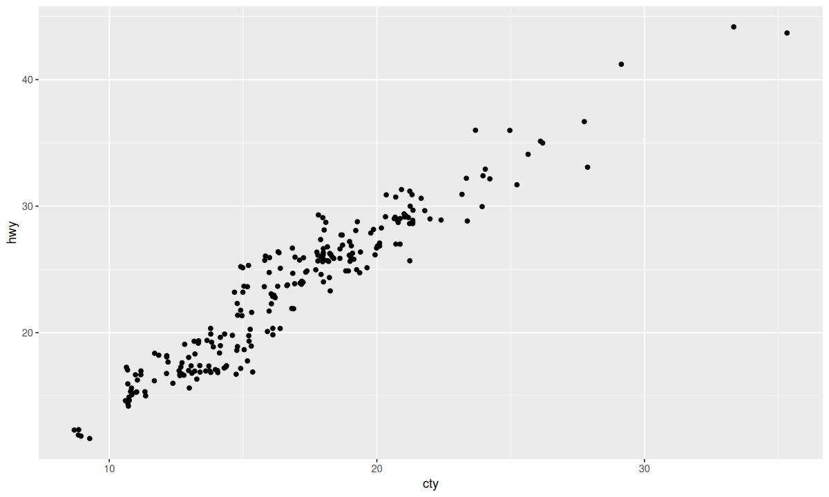
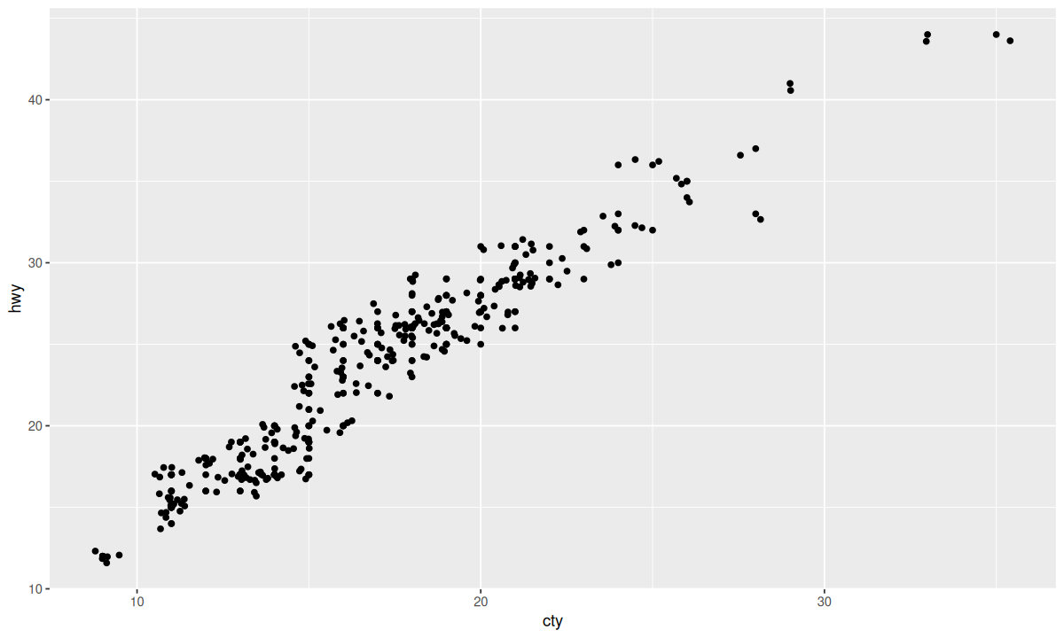
尽管添加随机性会损失图形的精确性,但可以大大提高图形的启发性。对比下面两张图:
1
2
3
4
5
| ggplot(data = mpg, mapping = aes(x = cty, y = hwy)) +
geom_point()
ggplot(data = mpg, mapping = aes(x = cty, y = hwy)) +
geom_point(position = "jitter")
|
可以使用 geom_jitter() 函数代替 position 参数来对抖动进行更详细的设置。
1
2
3
4
5
| ggplot(data = mpg, mapping = aes(x = cty, y = hwy)) +
geom_point() + geom_jitter(width = 0, height = 0)
ggplot(data = mpg, mapping = aes(x = cty, y = hwy)) +
geom_point() + geom_jitter(width = 0.5, height = 0.5)
|

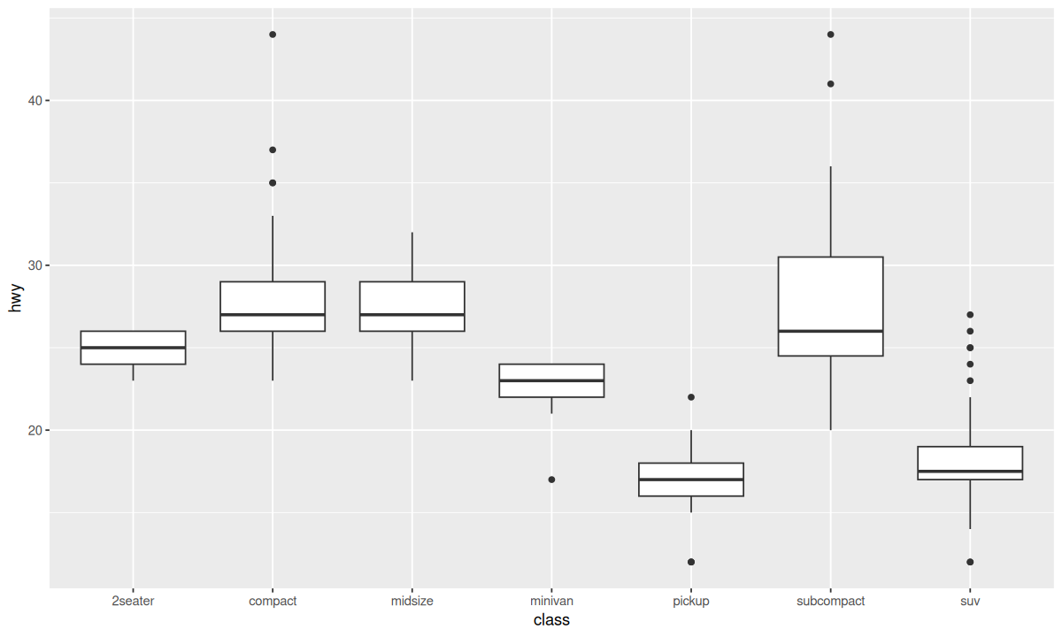
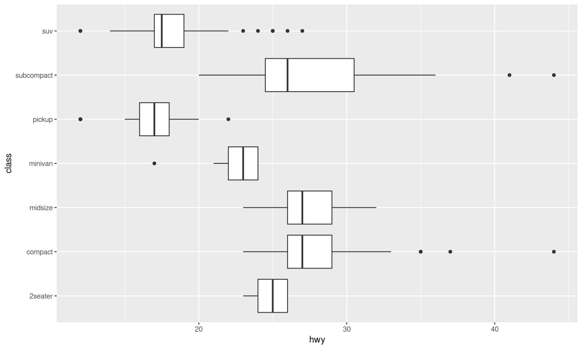
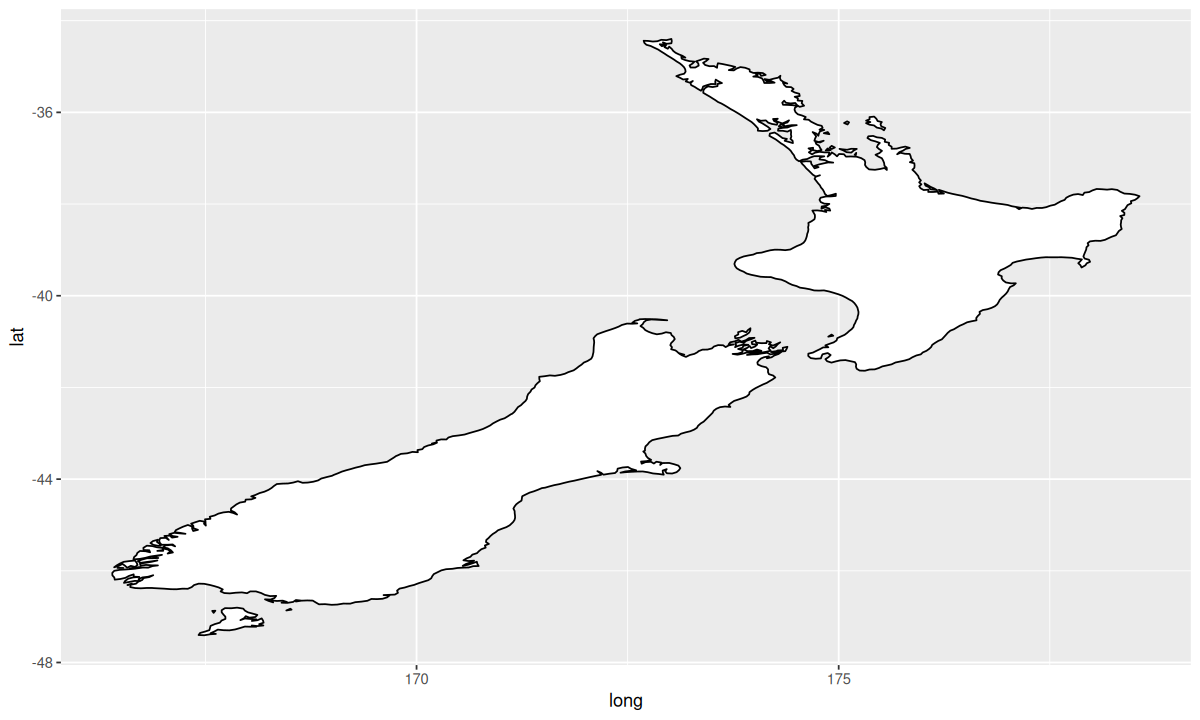
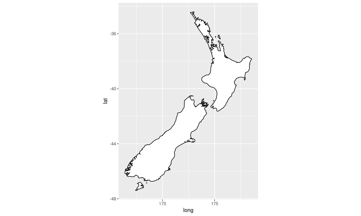
coord_flip() 函数可以交换 x 轴和 y 轴。coord_quickmap() 函数可以为地图设置合适的纵横比。coord_polar() 函数使用极坐标系。
1
2
3
4
5
| ggplot(data = mpg, mapping = aes(x = class, y = hwy)) +
geom_boxplot()
ggplot(data = mpg, mapping = aes(x = class, y = hwy)) +
geom_boxplot() +
coord_flip()
|
1
2
3
4
5
6
7
| nz <- map_data("nz")
ggplot(nz, aes(long, lat, group = group)) +
geom_polygon(fill = "white", color = "black")
ggplot(nz, aes(long, lat, group = group)) +
geom_polygon(fill = "white", color = "black") +
coord_quickmap()
|
 1
 2
 3
 4
 5
 6
 7
 8
 9
10
11
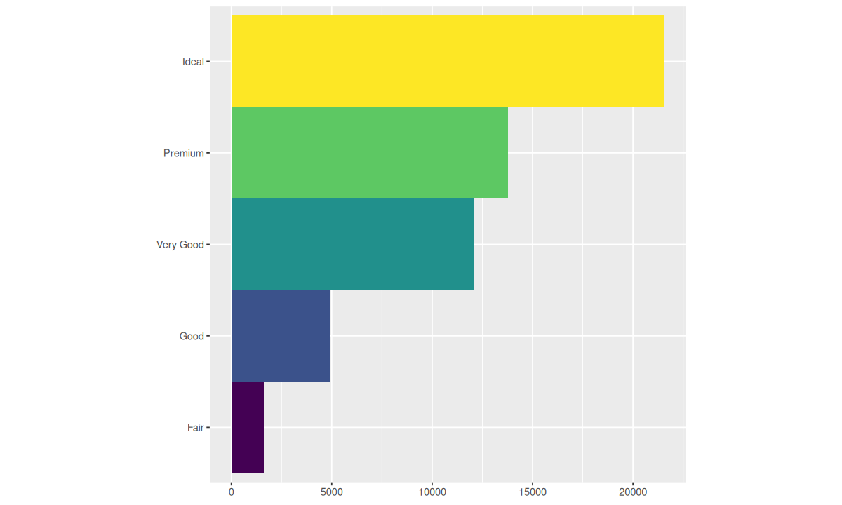
| bar <- ggplot(data = diamonds) +
geom_bar(
mapping = aes(x = cut, fill = cut),
show.legend = FALSE,
width = 1
) +
theme(aspect.ratio = 1) +
labs(x = NULL, y = NULL)
bar + coord_flip()
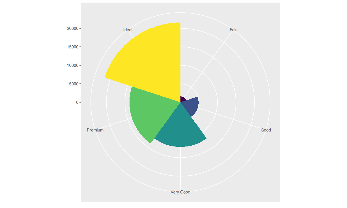
bar + coord_polar()
|
可以将任何图形精确地描述为数据集、几何对象、映射集合、统计变换、位置调整、坐标系和分面模式的一个组合,图形语法正是基于这样的深刻理解构建出来的:
1
2
3
4
5
6
7
8
| ggplot(data = <DATA>) +
<GEOM_FUNCTION>(
mapping = aes(<MAPPINGS>),
stat = <STAT>,
position = <POSITION>
) +
<COORDINATE_FUNCTION> +
<FACET_FUNCTION>
|