植体周炎预测模型：Logistic 回归分析及列线图模型

数据准备：使用 sample 函数对原始数据进行随机抽样，抽取 70% 的数据作为训练集（n=329），其余的作为测试集（n=141），抽样结果（训练集）保存在 sample.txt 文件中。
建立模型：使用 stats 程序包中的 glm 函数对训练集数据使用单因素和多因素 Logistic 回归分析，确定发生植体周炎的危险因素（P < 0.05）。用多因素 Logistic 回归分析的结果计算 OR 值，并借助 boot 程序包，使用 Bootstrap 法计算 OR 的 95% 置信区间。使用 rms 程序包建立列线图预测模型。
验证模型：分别借助 rms 程序包中的 calibrate 函数和 pROC 程序包中的 plot.roc 函数，使用 C-index 和校准曲线来检验模型的区分度和校准度。Logistic 回归的 C-index 即为 ROC 曲线下面积（AUC）。内部验证和外部验证分别使用训练集和测试集数据进行。

模型建立

准备工作

导入需要用到的 R 程序包并导入数据：

1
2
3
4
5
6
7
8
9
# 导入 R 库
library(readxl)
library(writexl)
# library(lme4)
library(broom)
library(tidyverse)

# 导入数据
raw_data <- read_excel("data.xlsx")

根据需要预处理数据

 1
 2
 3
 4
 5
 6
 7
 8
 9
10
11
12
13
14
15
16
17
18
19
20
21
22
23
24
25
26
27
28
# 选择研究变量
data <- raw_data[, c(-1, -2, -3, -10, -17, -18, -20)]
data$年龄 <- raw_data$修复体戴入日期 - raw_data$出生日期

# 计数数据
names.count <- c("吸烟", "性别", "修复体材料", "骨吸收情况", "分期", "分级",
                 "颌位", "牙位", "种植系统", "植骨手术明细", "用膜明细", "缝合方式")
names.all <- colnames(data)[-which(colnames(data) == "植体周炎")]

# 再次处理数据细节
data$口内植体数目 <- as.numeric(data$口内植体数目) # “口内植体数目” 原本是字符串，这里将其转换为数值
data[which(data$分级 == "B"), ]$分级 <- "b"         # 分级 B 和 b 相同
data[which(data$分级 == "a"), ]$分级 <- "b"         # 把分级里a合并到b里面
data[which(data$骨吸收情况 == "1/2"), ]$骨吸收情况 <- ">1/2"
data[which(as.numeric(data$修复体材料) >= 3), ]$修复体材料 <- 3 # 修复体材料 3 以后都合并为一类

# 处理错误数据
data[which(data$吸烟 == 2), ]$吸烟 <- 0
data[which(is.na(data$种植系统)), ]$种植系统 <- 1
data[which(is.na(data$用膜明细)), ]$用膜明细 <- 1

# 去除有缺失值的病例
data <- data[complete.cases(data), ]

# 计数数据转成因子型变量
for (name in names.count) {
    data[[name]] <- factor(data[[name]])
}

现在准备好的数据储存在 data 变量中。

 1
 2
 3
 4
 5
 6
 7
 8
 9
10
11
12
13
14
#> # A tibble: 6 × 23
#>   吸烟  种植前空腹血糖 性别  修复体材料 口内植体数目 骨吸收情况 分期  分级 
#>   <fct>          <dbl> <fct> <fct>             <dbl> <fct>      <fct> <fct>
#> 1 0               4.9  1     1                     4 <1/3       3     b    
#> 2 0               4.9  1     1                     4 1/3-1/2    3     b    
#> 3 0               5.98 1     1                     3 <1/3       3     c    
#> 4 0               4.89 2     1                     7 1/3-1/2    3     c    
#> 5 0               4.89 2     1                     7 植体       3     c    
#> 6 0               4.89 2     1                     7 1/3-1/2    4     c    
#> # ℹ 15 more variables: 颌位 <fct>, 牙位 <fct>, `角化组织宽度（mm）` <dbl>,
#> #   `维护周期（月）` <dbl>, 平均复查周期 <dbl>, 种植系统 <fct>, 植体直径 <dbl>,
#> #   植体长度 <dbl>, 植骨手术明细 <fct>, 用膜明细 <fct>, 缝合方式 <fct>,
#> #   `穿龈角度（近中）` <dbl>, `穿龈角度（远中）` <dbl>, 植体周炎 <dbl>,
#> #   年龄 <drtn>

训练集和测试集

通过以下代码随机选取 7/10 的数据作为训练集，并将抽样方案保存在 sample.txt 文件中。

1
2
smp <- sample(seq_len(nrow(data)), round(nrow(data) * 0.7))
write(smp, file = "sample.txt")

代码编写过程中可能需要多次运行代码，为保持多次运行之间的一致性，在选取合适的抽样（单因素 Logistic 回归）后，之后的抽样选取就通过读取 sample.txt 文件完成。

1
2
3
4
# 随机抽取训练集，其他作为测试集
smp <- scan(file = "sample.txt")
data.train <- data[smp, ]
data.test <- data[-smp, ]

单因素 Logistic 回归

使用 glm 函数，对训练集数据的每个预测变量进行单因素分析，获取 P 值，并选出 P < 0.05 的预测变量（抽样的不同会对这一步造成较大影响）。

 1
 2
 3
 4
 5
 6
 7
 8
 9
10
11
12
13
14
15
16
p.values <- data.frame()
names.selected <- c()
for (name in names.all) {
  f <- as.formula(paste(c("植体周炎", paste(c("`", name, "`"), collapse = "")), collapse = "~"))
  model.tmp <- glm(f, data = data.train, family = binomial())
  additions <- summary(model.tmp)$coefficients[-1, 4]
  if (is.null(names(additions))) {
    names(additions) <- paste(name, levels(data.train[[name]])[-1], sep = "")
  }

  p.values <- rbind(p.values, data.frame("P value" = additions))
  if (any(additions < 0.05)) {
    names.selected <- c(names.selected, name)
  }
}
names.selected

1
2
#> [1] "修复体材料"     "骨吸收情况"     "分级"           "维护周期（月）"
#> [5] "平均复查周期"

根据单因素 Logistic 回归的结果，这次抽样选出的危险因素（P < 0.05）为：“修复体材料”，“骨吸收情况”，“分级”，“维护周期（月）”和“平均复查周期”。

多因素 Logistic 回归

用单因素 Logistic 回归筛选出的危险因素，同样使用 glm 函数，进行多因素 Logistic 回归分析。

1
2
3
4
5
6
7
8
9
names.05 <- names.selected
f.05 <- as.formula(paste(collapse = "~",
   c(
     "植体周炎",
     paste(collapse = "", c("`", paste(names.05, collapse = "`+`"), "`"))
     )
))
model.05 <- glm(f.05, data = data.train, family = binomial())
summary(model.05)

 1
 2
 3
 4
 5
 6
 7
 8
 9
10
11
12
13
14
15
16
17
18
19
20
21
22
23
24
25
#> 
#> Call:
#> glm(formula = f.05, family = binomial(), data = data.train)
#> 
#> Coefficients:
#>                   Estimate Std. Error z value Pr(>|z|)    
#> (Intercept)       -5.26989    0.72909   -7.23  4.9e-13 ***
#> 修复体材料2       -0.07740    0.41125   -0.19  0.85072    
#> 修复体材料3        0.95364    0.52022    1.83  0.06678 .  
#> 骨吸收情况>1/2     2.81191    0.63639    4.42  9.9e-06 ***
#> 骨吸收情况1/3-1/2  0.66028    0.44389    1.49  0.13689    
#> 骨吸收情况植体     1.12159    0.52408    2.14  0.03235 *  
#> 分级c              1.08745    0.44902    2.42  0.01544 *  
#> `维护周期（月）`   0.02031    0.00576    3.52  0.00042 ***
#> 平均复查周期       0.01974    0.00941    2.10  0.03593 *  
#> ---
#> Signif. codes:  0 '***' 0.001 '**' 0.01 '*' 0.05 '.' 0.1 ' ' 1
#> 
#> (Dispersion parameter for binomial family taken to be 1)
#> 
#>     Null deviance: 283.80  on 328  degrees of freedom
#> Residual deviance: 219.58  on 320  degrees of freedom
#> AIC: 237.6
#> 
#> Number of Fisher Scoring iterations: 6

注意这里构建公式的方法：先使用加了 collapse 参数的 paste 函数将 names.05 拼接成字符串形式的“公式”，再通过 as.formula 方法，将字符串转换为公式。

OR 及 OR 的 95% 置信区间

在 R 中，可以使用 exp(coef(model)) 计算比值比（OR）。

既可以借助 boot 程序包，使用 Bootstrap 法计算 OR 及其 95% 置信区间，也可以直接使用confint 函数。

Bootstrap 法

为了控制更多的细节，这里使用 boot 程序包的 boot 函数计算 OR，并使用同属于 boot 程序包的 boot.ci 函数计算置信区间。

 1
 2
 3
 4
 5
 6
 7
 8
 9
10
11
12
13
14
15
16
17
18
19
20
21
22
23
24
25
26
library(boot)
set.seed(1645248416) # unclass(Sys.time())

# 计算 OR 值的函数
st.boot <- function(data, indices) {
  model <- glm(f.05, data[indices, ], family = binomial())
  return(exp(coef(model)))
}

# 运行 Bootstrap 计算 OR
results <- boot(data.train, statistic = st.boot, R = 1000)

ci <- matrix(nrow = length(results$t0), ncol = 2)
colnames(ci) <- c("2.5%", "97.5%")
rownames(ci) <- names(results$t0)
for (i in seq_len(length(results$t0))) {
  n <- boot.ci(boot.out = results, conf = 0.95, type = "bca", index = i)
  ci[i, ] <- n$bca[c(4, 5)]
}

table2.05 <- data.frame(
  "OR" = results$t0,
  "OR.CI" = ci,
  "P值" = tidy(model.05)$p.value
)
head(table2.05)

1
2
3
4
5
6
7
#>                          OR OR.CI.2.5. OR.CI.97.5.       P值
#> (Intercept)        0.005144   0.001077     0.02295 4.901e-13
#> 修复体材料2        0.925524   0.365046     2.13859 8.507e-01
#> 修复体材料3        2.595143   0.856581     7.63863 6.678e-02
#> 骨吸收情况>1/2    16.641733   4.311440    62.61887 9.938e-06
#> 骨吸收情况1/3-1/2  1.935325   0.718117     4.88898 1.369e-01
#> 骨吸收情况植体     3.069725   0.762045     8.27774 3.235e-02

`confint` 函数

1
2
3
4
5
6
table_simple <- data.frame(
  "OR" = exp(coef(model.05)),
  "OR.CI" = exp(confint(model.05)),
  "P值" = tidy(model.05)$p.value
)
head(table_simple)

1
2
3
4
5
6
7
#>                          OR OR.CI.2.5.. OR.CI.97.5..       P值
#> (Intercept)        0.005144    0.001112      0.01965 4.901e-13
#> 修复体材料2        0.925524    0.403301      2.04682 8.507e-01
#> 修复体材料3        2.595143    0.913069      7.12754 6.678e-02
#> 骨吸收情况>1/2    16.641733    4.901419     60.79632 9.938e-06
#> 骨吸收情况1/3-1/2  1.935325    0.811607      4.67088 1.369e-01
#> 骨吸收情况植体     3.069725    1.063397      8.47141 3.235e-02

OR 和 P 值与之前的结果相同，但置信区间有少许差别。

列线图预测模型

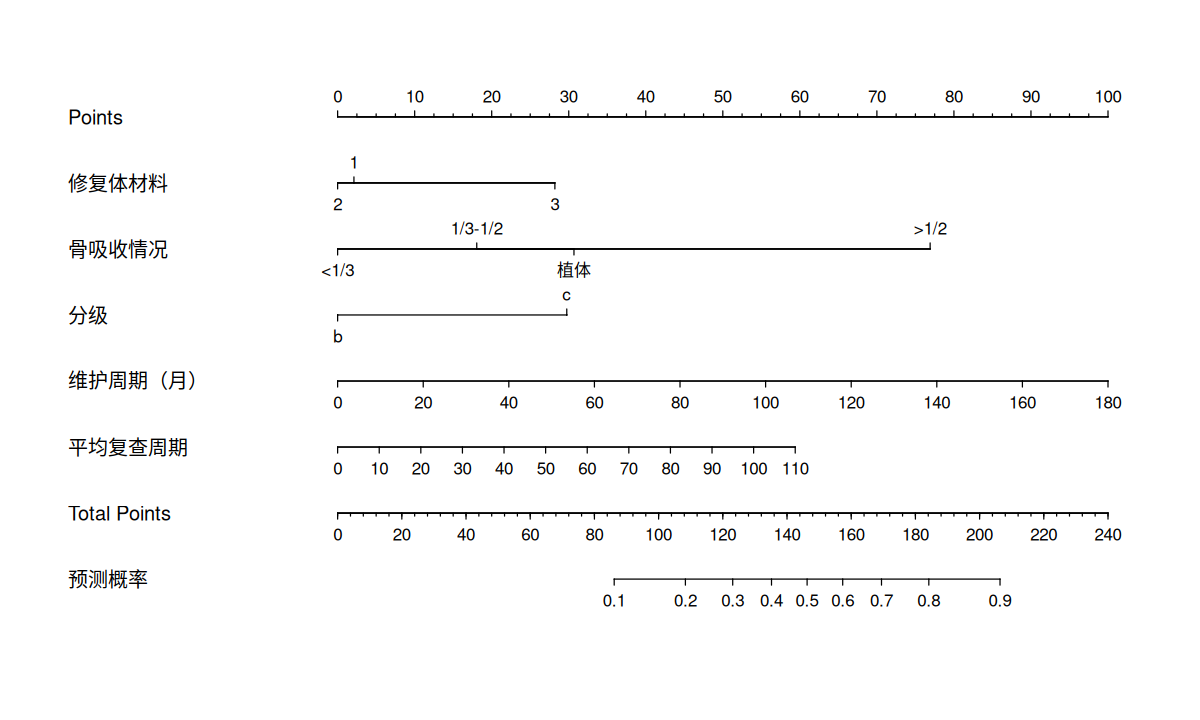
rms 程序包提供了用来建立列线图预测模型的函数。

1
2
3
4
5
6
7
library(rms)

# 使用训练集建立列线图预测模型
fit.train <- lrm(f.05, data.train, x = TRUE, y = TRUE)
ddist.train <- datadist(data.train)
options(datadist = ddist.train)
plot(nomogram(fit.train, fun = plogis, lp = FALSE, funlabel = "预测概率"))

数据验证

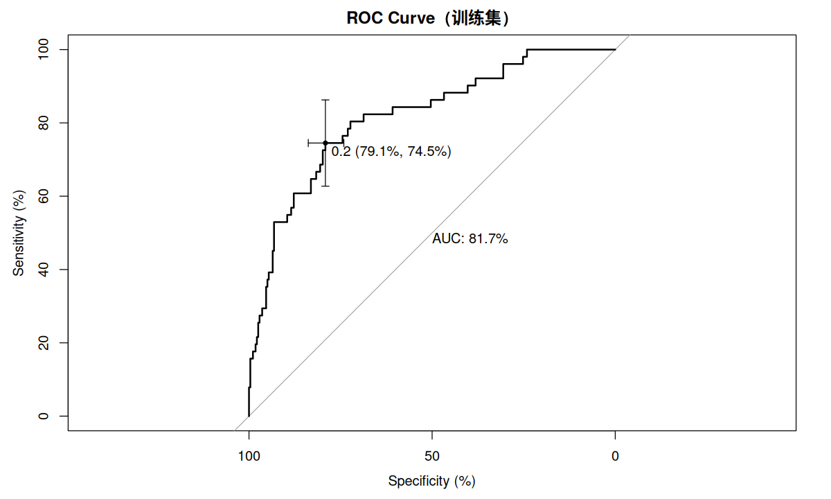
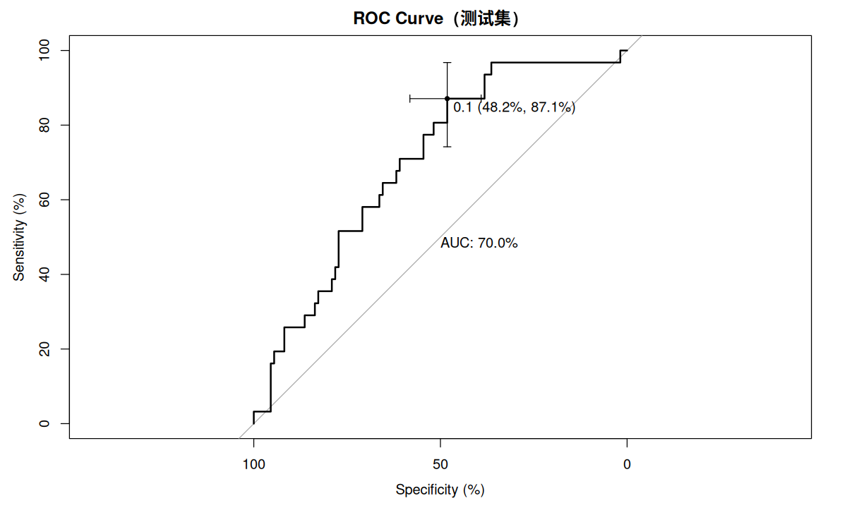
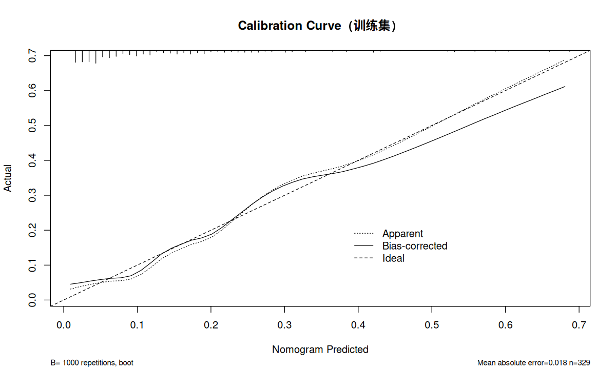
数据验证分为内部验证和外部验证。这里使用测试集进行外部验证，内部验证在训练集上进行。在内部验证和外部验证中，都分别通过 ROC 曲线和列线图校准曲线检验数据的区分度和校准度。

ROC 曲线

特异度和敏感度
由FeanDoe - Modified version from Walber's Precision and Recall <a class="external free" href="https://commons.wikimedia.org/wiki/File:Precisionrecall.svg">https://commons.wikimedia.org/wiki/File:Precisionrecall.svg</a>，CC BY-SA 4.0，链接

ROC 曲线全称受试者工作特征曲线 （receiver operating characteristic curve），又称为感受性曲线（sensitivity curve），曲线上每个点反映着对同一信号刺激的感受性。
ROC 曲线的横轴为特异度（specificity），即真阴性率（true negative rate，TNR）；纵轴为敏感度（sensitivity），即真阳性率（true postive rate，TPR）、召回率（Recall）。

$$Specificity=TNR=\frac{TN}{N}=\frac{TN}{TN+FP}
\,.$$

$$Sensitivity=TPR=Recall=\frac{TP}{P}=\frac{TP}{TP+FN}
\,.$$

AUC 全称曲线下面积（Area Under Curve），在 Logistic 回归中，AUC 等同于 C-index（concordance index，一致性指数），可以直观的评价模型的好坏，值越大越好。

使用 ROC 曲线检验数据的区分度，pROC 程序包提供了这里所需要的函数，其中 plot.roc 用于绘制 ROC 曲线，ci.auc 用于获取 AUC 的置信区间。

1
library(pROC)

1
2
3
4
5
6
7
8
pre.train <- predict(model.05, data.train, type = c("response"))
p.roc.train <- plot.roc(data.train$植体周炎, pre.train,
                        main = "ROC Curve（训练集）", percent = TRUE,
                        print.auc = TRUE,
                        ci = TRUE, of = "thresholds",
                        thresholds = "best",
                        print.thres = "best")
ci.auc(p.roc.train)

1
#> 95% CI: 75.2%-88.2% (DeLong)

1
2
3
4
5
6
7
8
pre.test <- predict(model.05, data.test, type = c("response"))
p.roc.test <- plot.roc(data.test$植体周炎, pre.test,
                        main = "ROC Curve（测试集）", percent = TRUE,
                        print.auc = TRUE,
                        ci = TRUE, of = "thresholds",
                        thresholds = "best",
                        print.thres = "best")
ci.auc(p.roc.test)

1
#> 95% CI: 60.2%-79.8% (DeLong)

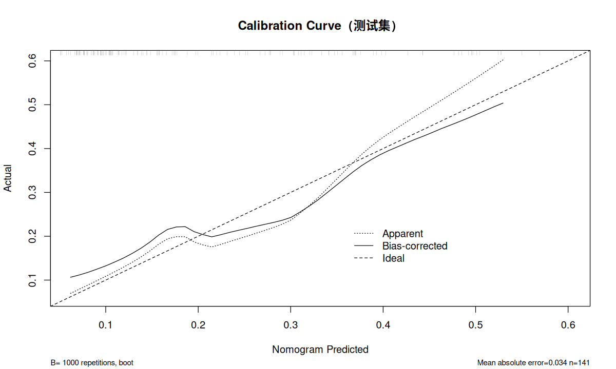
训练集 AUC 达 81.7%（95%CI：75.16%-88.25%），测试集 AUC 为 70.0%（95%CI：60.24%-79.76%），提示列线图模型区分度良好。

列线图校准曲线

使用列线图校准曲线检验数据的校准度。绘制列线图校准曲线用到的 calibrate 也是 rms 包中的函数。这里使用 Bootstrap 法（method = "boot"），重复 1000 次（B = 1000）。其他常用的 method 还有 "crossvalidation"、".632" 及 "randomization"。

1
2
3
4
5
cal_train <- calibrate(fit.train,  method = "boot", B = 1000)
plot(cal_train,
     xlab = "Nomogram Predicted",
     ylab = "Actual",
     main = "Calibration Curve（训练集）")

1
2
3
4
5
6
7
8
9
fit.test <- lrm(f.05, data.test, x = TRUE, y = TRUE)
ddist.test <- datadist(data.test)
options(datadist = ddist.test)

cal_test <- calibrate(fit.test,  method = "boot", B = 1000)
plot(cal_test,
     xlab = "Nomogram Predicted",
     ylab = "Actual",
     main = "Calibration Curve（测试集）")

通过校验曲线可以看出训练集和测试集的预测值与实际值基本一致。

植体周炎预测模型：Logistic 回归分析及列线图模型

特异度和敏感度