2024-10-06 R tips
数据框和列表均可以直接添加新项:
1
2
3
4
5
6
| df <- data.frame(
a = c(1, 2, 3),
b = c("b")
)
df$c <- c("a", "b", "c")
df
|
1
2
3
4
| #> a b c
#> 1 1 b a
#> 2 2 b b
#> 3 3 b c
|
1
2
3
4
5
6
| lt <- list(
a <- matrix(1:10, nrow = 2),
b <- "test_string"
)
lt[["c"]] <- "additional entry"
lt
|
 1
 2
 3
 4
 5
 6
 7
 8
 9
10
| #> [[1]]
#> [,1] [,2] [,3] [,4] [,5]
#> [1,] 1 3 5 7 9
#> [2,] 2 4 6 8 10
#>
#> [[2]]
#> [1] "test_string"
#>
#> $c
#> [1] "additional entry"
|
向量可以使用 c() 或 append() 插入新项:
1
2
3
4
5
6
| vc <- c(1, 2, 3)
c(vc, 4)
c(4, vc)
append(vc, after = 0, 0) # 在最前面插入
append(vc, after = length(vc), 4) # 在最后面插入
append(vc, 4) # 默认在最后面插入
|
1
2
3
4
5
| #> [1] 1 2 3 4
#> [1] 4 1 2 3
#> [1] 0 1 2 3
#> [1] 1 2 3 4
#> [1] 1 2 3 4
|
对于列表,$ 和 [[]] 几乎一样,返回值是子项;而 [] 的返回值则是子集,类型仍然是列表。
 1
 2
 3
 4
 5
 6
 7
 8
 9
10
11
12
13
| lt <- list(
a = c(1, 2, 3),
b = "string"
)
cat("lt$a:\n")
lt$a
cat("lt[[\"a\"]]:\n")
lt[["a"]]
cat("lt[\"a\"]:\n")
lt["a"]
cat("lt[1:2]:\n")
lt[1:2]
|
 1
 2
 3
 4
 5
 6
 7
 8
 9
10
11
12
13
14
| #> lt$a:
#> [1] 1 2 3
#> lt[["a"]]:
#> [1] 1 2 3
#> lt["a"]:
#> $a
#> [1] 1 2 3
#>
#> lt[1:2]:
#> $a
#> [1] 1 2 3
#>
#> $b
#> [1] "string"
|
除了 %>%,R 语言(4.1+)提供了原生的管道运算符 |>。在 Rstudio 中,通过 “Tools” → “Global Options…” → “Editing” → “Use native pipe operator, |> (requires R 4.1+)” 来启用。
默认快捷键是 Ctrl+Shift+m。
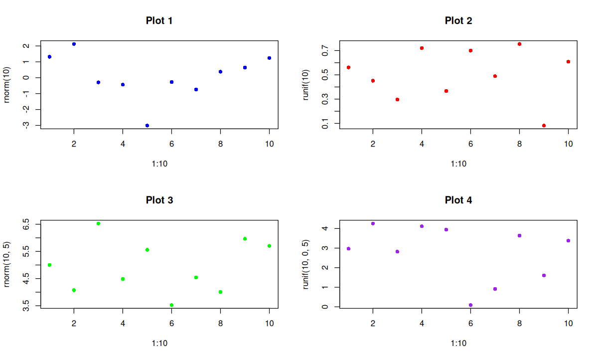
同时绘制几个 plot:
 1
 2
 3
 4
 5
 6
 7
 8
 9
10
| # 设置绘图区域为 2 行 2 列
par(mfrow = c(2, 2))
plot(1:10, rnorm(10), main = "Plot 1", col = "blue", pch = 16)
plot(1:10, runif(10), main = "Plot 2", col = "red", pch = 16)
plot(1:10, rnorm(10, 5), main = "Plot 3", col = "green", pch = 16)
plot(1:10, runif(10, 0, 5), main = "Plot 4", col = "purple", pch = 16)
# 恢复默认的单个图形布局
par(mfrow = c(1, 1))
|
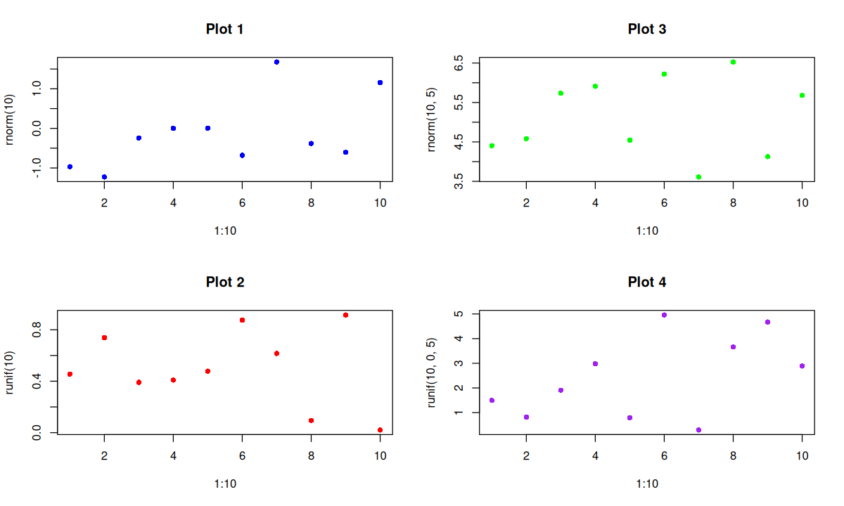
使用 mfcol 参数会先填充列:
 1
 2
 3
 4
 5
 6
 7
 8
 9
10
| # 设置绘图区域为 2 列 2 行
par(mfcol = c(2, 2))
plot(1:10, rnorm(10), main = "Plot 1", col = "blue", pch = 16)
plot(1:10, runif(10), main = "Plot 2", col = "red", pch = 16)
plot(1:10, rnorm(10, 5), main = "Plot 3", col = "green", pch = 16)
plot(1:10, runif(10, 0, 5), main = "Plot 4", col = "purple", pch = 16)
# 恢复默认的单个图形布局
par(mfrow = c(1, 1))
|
par():设置一些重要参数plot(): 基本的绘图函数,或用于为其他一些函数创建“画板”rasterImage():绘制像素图像text():在任意位置绘制文本title():绘制标题、副标题以及 X、Y 轴标签。
- 注意:在
for 循环中,需要显式地使用 print() 函数来显示图像。
- 使用
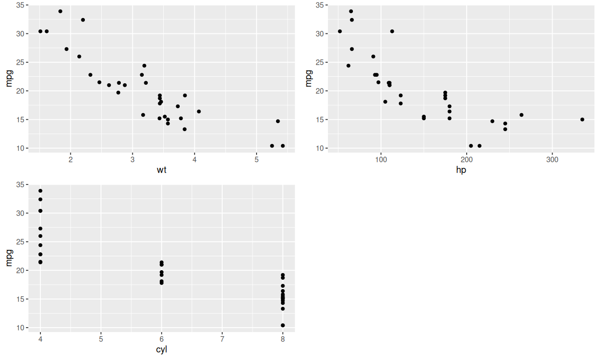
patchwork 包可以方便的用 +、|、/ 来排列图像。 cowplot 与 ggplot2 集成良好。函数 plot_grid() 可用来布局,功能类似 gridExtra::grid.arrange(),但语法更加简洁。
 1
 2
 3
 4
 5
 6
 7
 8
 9
10
11
12
13
14
| library(ggplot2)
library(cowplot)
plot1 <- ggplot(mtcars, aes(x = wt, y = mpg)) + geom_point()
plot2 <- ggplot(mtcars, aes(x = hp, y = mpg)) + geom_point()
plot3 <- ggplot(mtcars, aes(x = cyl, y = mpg)) + geom_point()
plot_list <- list(plot1, plot2, plot3)
# 通过 do.call 合并 plot_list
combined_plot <- do.call(plot_grid, c(plot_list, ncol = 2))
combined_plot
# 也可以直接用 plotlist 参数
plot_grid(plotlist = plot_list, ncol = 2)
|

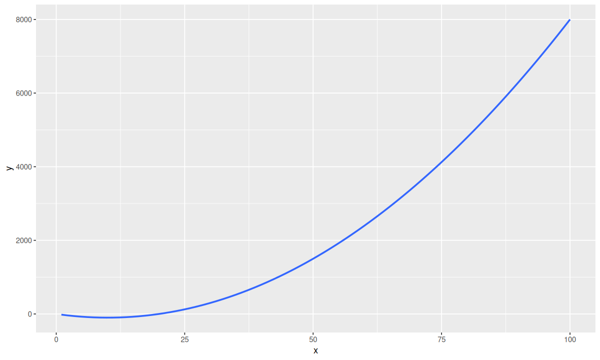
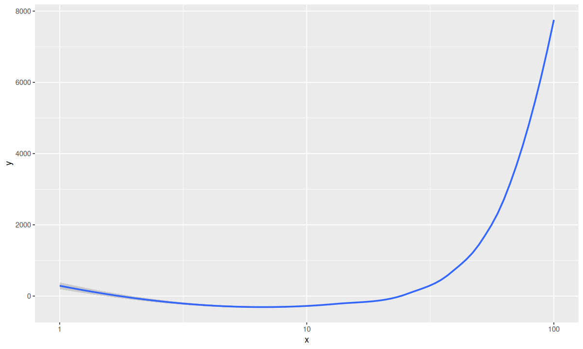
coord_fixed(ratio = 1):设置 x、y 坐标比例为 1:1。scale_x_continuous(limits = c(2, 5)):设置横坐标范围。scale_x_continuous(breaks = c(0, 100, 200, 300, 350), labels = c(0, 100, 200, 300, "infinite")):设置刻度线和标签。scale_x_continuous(transform = "log10")(trans 已被废弃):设置坐标轴转换。Built-in transformations include “asn”, “atanh”, “boxcox”, “date”, “exp”, “hms”, “identity”, “log”, “log10”, “log1p”, “log2”, “logit”, “modulus”, “probability”, “probit”, “pseudo_log”, “reciprocal”, “reverse”, “sqrt” and “time”.
 1
 2
 3
 4
 5
 6
 7
 8
 9
10
11
12
13
14
| # 注意命名方式,scale_x_continuous 会自动查找 transform_xxx 函数
transform_log10 <- scales::trans_new(
name = "trans_log10",
transform = function(x) log10(x),
inverse = function(x) 10 ^ x,
breaks = function(limits) 10 ^ pretty(log10(limits))
)
xs <- seq(1, 100, by = 0.2)
ggplot(data.frame(x = xs, y = xs ^ 2 - 20 * xs)) +
geom_smooth(mapping = aes(x, y))
ggplot(data.frame(x = xs, y = xs ^ 2 - 20 * xs)) +
geom_smooth(mapping = aes(x, y)) +
scale_x_continuous(transform = "log10")
|